Visualizing rings in social network

Let's say we were assigned the task of identifying the shortest path of sending a message in a social network of friends, how do we go about in deciding which persons to send the message to:

Algorithm:

1. extract all friends (or interactions)

2. extract friends for each friend (for example if you are friends with A, extract all the friends of A)

3. find all the friends who are common to you and your friend

4. apply a clustering algorithm where distance between centre of clusters is maximised while distance between points is minimised

and we have the rings in a social network.

Social network rings

Visualizing with ggplot

ggplot presents with an extremely powerful data visualization capability through R.

There are many different variations of graphs that one could come up with using this package.

Below, is a demo of a visualisation that could give the micro level detail of a CS network at a half hour interval for all the days of week.

All it takes is 3 lines of code with dummy data

Interval level detail of forecast versus actuals

data$interval=as.factor(data$interval)

data$day=factor(data$day,levels=c("Saturday","Friday","Thursday","Wednesday","Tuesday","Monday","Sunday"))

ggplot(data,aes(interval2,day,color=diff))+facet_grid(site~channel)+geom_tile()+theme_bw()+scale_fill_gradient(low="red", high="yellow")

Scraping websites to identify if one's logo exists

This post is a demo for the project in which one had to scrape websites to see if they accept cards from one of the credit card companies.

Typically websites have the logo of he credit card company if they accept the card in their payments page.

Manually, if a person would have to do this task, he would open each link and go to the payments page and then check if there is the related logo.

However, if a machine were to do this task, as per the code I have written it would go through the following steps:

1. Open the webpage to be tested

For example: link='http://www.listphile.com/Fortune_500_Logos/list'
webpage=urllib.urlopen(link).read()

2. Look for all the href links that link to other pages, for now, let's assume that we directly land on the payments page

3. Find all logos existing in that page

findlogo=re.compile('<a href="/Fortune_500_Logos/(.*)"><img alt="Thumb" height="62" src="(.*)" title="(.*)')
findnewlogo=re.findall(findlogo,webpage)

4. Extract logos from the website

for i in xrange(100):
urllib.urlretrieve("http://www.listphile.com"+findnewlogo[i][1], "local drive".png")


5. Resize all the logos extacted so that they all can be compared
im1=Image.open("E:/amex/logo comparison/"+findnewlogo[j][0]+".png")
im1.resize((30,30))

6. Compute the difference between extracted logo and the logo of the company we wanted to check for match

h = ImageChops.difference(im11, im22).histogram()
difference=math.sqrt(reduce(operator.add,map(lambda h, i: h*(i**2), h, range(256))))

7. Flag if there is a difference


In this way, one could reduce a lot of manual intervention.

However, the caveat here is that, there might be cases when the program does not even land in payments' page.
This can be identified by raising a flag when the number of links within a webpage are too large that if the program did not find the payments' page, one needs to have a manual check for the respective website

Getting into Kaggle Top 20% in one evening

Kaggle.com is one of the top platform for data scientists to test their skills against the best and ranking among the top on its competitions is one of the hardest tasks to accomplish.

However, the gap between the top performers is so small and a minute improvement in score possibly follows the 80-20 distribution where one can reach the top 20% scores in reasonably small time, however achieving the top might take a lot more effort.

However, the top scores would face another problem -

Implementation in production - netflix paid $1Mn, in their competition, however, the models were so very complicated that it found hard to implement the winning model.


This post describes my results in achieving among the top 20% scores with

1. Feature engineering
2. Single GBM model

Feature engineering represents the modification of variables by either reshaping them or
GBM is quite possibly the best performing individual model among the many other machine learning techniques.

Competition 1: Carvana

Carvana had ~20 variables with 15 categorical & 5 continuous variables with the dependent variable being if the car was a bad buy or not.

Among the 15 categorical variables, 10 had not more than 5 factors, while 5 had a lot of factors (~1000 levels).

Given these were factors, they could not get directly into the regression problem.

So they were reshaped in a way where the factor was transformed into a variable dummy and given a binary value of whether it is a 1 or a 0.

That was pretty much it, we have ~100 variables and ~70K rows .

On top of this dataset, I have applied a GBM model with 1000 trees and voila, I was in the top 20% in one evening's effort out of ~600 participants.

Competition 2: Detecting influencers in social network

This competition was around identifying if A has more influence in a social network when compared to B.
Dataet was provided with features like # of followers, mentions, retweets, posts and other network features for the two users, with each pair of A, B in a new row.

Feature engineering for this dataset was around taking the difference of # of followers, mentions, posts etc., for A, B and also taking the ratio.

and voila this resulted in 12th position in the competition!!

TSP art

TSP stands for Travelling Sales Man problem, which minimises the cost of travelling through all the cities by minimising the distance travelled.

TSP art is essentially taking a picture and converting it into a scatterplot and then connecting the dots in scatterplot by lines to produce a not so smooth image, but aesthetically good one for sure.

Some examples of TSP art is here

Some of the applications of this work could potentially be around making the images move - as in, eyes, arms, legs can be segmented once we take images and make them learn features to understand different body parts. Once this is done, an image can move as per one's wish!


Here's the workings of creating TSP art:

Step1:  Converting image into scatterplot

1. Load image
2. Extract pixel values for each x & y points of the image
3. Extract pixel values of each x & y where the pixel value is greater than a certain threshold

and we have the scatterplot for an image

Step 2: create TSP while assumign the scatterplot points as cities

1. Assume each data point of the image as a city with x & y co-ordinates
2. Identify the path through which a salesman can go through each city while minimising the distance travelled
3. Plot the path


Here's the output of the above steps.

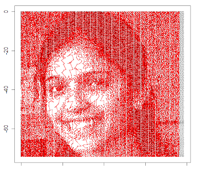TSP art

The code is here:
 import Image
 image = Image.open("folder").convert("L")
 pix=image.load()
 outfile=open('folder','w')
 for i in xrange(image.size[0]):
for j in xrange(image.size[1]):
outData='%s\t%s\t%s' % (i,j,data[i][j])
outfile.write(outData + '\n')

 train <- read.table("folder",header=TRUE, sep=",", na.strings="NA", dec=".", strip.white=TRUE)
 newtrain=train[train$rev_pix>150,]
 plot(newtrain$x,-newtrain$y,data=newtrain)

library(geosphere)
library(TSP)



newtrain$pixel=NULL
newtrain$rev_pixel=NULL

newtrain=newtrain/3

newtrain2=newtrain



newtrain3=newtrain2[1:1000,]

d=dist(newtrain3)

tsp=TSP(d)


tsp <- insert_dummy(tsp, label = "cut")


tour <- solve_TSP(tsp, method = "nearest_insertion")
path1 <- cut_tour(tour, "cut")


newtrain4=newtrain2[1001:2000,]

d=dist(newtrain4)

tsp=TSP(d)


tsp <- insert_dummy(tsp, label = "cut")


tour <- solve_TSP(tsp, method = "nearest_insertion")
path2 <- cut_tour(tour, "cut")


newtrain5=newtrain2[2001:3000,]

d=dist(newtrain5)

tsp=TSP(d)


tsp <- insert_dummy(tsp, label = "cut")


tour <- solve_TSP(tsp, method = "nearest_insertion")
path3 <- cut_tour(tour, "cut")


newtrain6=newtrain2[3001:4000,]

d=dist(newtrain6)

tsp=TSP(d)


tsp <- insert_dummy(tsp, label = "cut")


tour <- solve_TSP(tsp, method = "nearest_insertion")
path4 <- cut_tour(tour, "cut")


newtrain7=newtrain2[4001:5000,]

d=dist(newtrain7)

tsp=TSP(d)


tsp <- insert_dummy(tsp, label = "cut")


tour <- solve_TSP(tsp, method = "nearest_insertion")
path5 <- cut_tour(tour, "cut")


newtrain8=newtrain2[5001:6000,]

d=dist(newtrain8)

tsp=TSP(d)


tsp <- insert_dummy(tsp, label = "cut")


tour <- solve_TSP(tsp, method = "nearest_insertion")
path6 <- cut_tour(tour, "cut")


newtrain9=newtrain2[6001:7000,]

d=dist(newtrain9)

tsp=TSP(d)


tsp <- insert_dummy(tsp, label = "cut")


tour <- solve_TSP(tsp, method = "nearest_insertion")
path7 <- cut_tour(tour, "cut")


newtrain10=newtrain2[7001:8000,]

d=dist(newtrain10)

tsp=TSP(d)


tsp <- insert_dummy(tsp, label = "cut")


tour <- solve_TSP(tsp, method = "nearest_insertion")
path8 <- cut_tour(tour, "cut")


newtrain11=newtrain2[8001:9000,]

d=dist(newtrain11)

tsp=TSP(d)


tsp <- insert_dummy(tsp, label = "cut")


tour <- solve_TSP(tsp, method = "nearest_insertion")
path9 <- cut_tour(tour, "cut")


newtrain12=newtrain2[9001:10000,]

d=dist(newtrain12)

tsp=TSP(d)


tsp <- insert_dummy(tsp, label = "cut")


tour <- solve_TSP(tsp, method = "nearest_insertion")
path10 <- cut_tour(tour, "cut")


newtrain13=newtrain2[10001:11000,]

d=dist(newtrain13)

tsp=TSP(d)


tsp <- insert_dummy(tsp, label = "cut")


tour <- solve_TSP(tsp, method = "nearest_insertion")
path11 <- cut_tour(tour, "cut")


newtrain14=newtrain2[11001:12000,]

d=dist(newtrain14)

tsp=TSP(d)


tsp <- insert_dummy(tsp, label = "cut")


tour <- solve_TSP(tsp, method = "nearest_insertion")
path12 <- cut_tour(tour, "cut")

newtrain15=newtrain2[12001:13000,]

d=dist(newtrain15)

tsp=TSP(d)


tsp <- insert_dummy(tsp, label = "cut")


tour <- solve_TSP(tsp, method = "nearest_insertion")
path13 <- cut_tour(tour, "cut")

newtrain16=newtrain2[13001:14000,]

d=dist(newtrain16)

tsp=TSP(d)


tsp <- insert_dummy(tsp, label = "cut")


tour <- solve_TSP(tsp, method = "nearest_insertion")
path14 <- cut_tour(tour, "cut")

newtrain17=newtrain2[14001:15000,]

d=dist(newtrain17)

tsp=TSP(d)


tsp <- insert_dummy(tsp, label = "cut")


tour <- solve_TSP(tsp, method = "nearest_insertion")
path15 <- cut_tour(tour, "cut")

newtrain18=newtrain2[15001:16000,]

d=dist(newtrain18)

tsp=TSP(d)


tsp <- insert_dummy(tsp, label = "cut")


tour <- solve_TSP(tsp, method = "nearest_insertion")
path16 <- cut_tour(tour, "cut")


newtrain19=newtrain2[16001:17000,]

d=dist(newtrain19)

tsp=TSP(d)


tsp <- insert_dummy(tsp, label = "cut")


tour <- solve_TSP(tsp, method = "nearest_insertion")
path17 <- cut_tour(tour, "cut")

newtrain20=newtrain2[17001:18000,]

d=dist(newtrain20)

tsp=TSP(d)


tsp <- insert_dummy(tsp, label = "cut")


tour <- solve_TSP(tsp, method = "nearest_insertion")
path18 <- cut_tour(tour, "cut")

newtrain21=newtrain2[18001:19000,]

d=dist(newtrain21)

tsp=TSP(d)


tsp <- insert_dummy(tsp, label = "cut")


tour <- solve_TSP(tsp, method = "nearest_insertion")
path19 <- cut_tour(tour, "cut")

newtrain22=newtrain2[19001:20000,]

d=dist(newtrain22)

tsp=TSP(d)


tsp <- insert_dummy(tsp, label = "cut")


tour <- solve_TSP(tsp, method = "nearest_insertion")
path20 <- cut_tour(tour, "cut")

newtrain23=newtrain2[20001:21000,]

d=dist(newtrain23)

tsp=TSP(d)


tsp <- insert_dummy(tsp, label = "cut")


tour <- solve_TSP(tsp, method = "nearest_insertion")
path21 <- cut_tour(tour, "cut")

newtrain24=newtrain2[21001:22000,]

d=dist(newtrain24)

tsp=TSP(d)


tsp <- insert_dummy(tsp, label = "cut")


tour <- solve_TSP(tsp, method = "nearest_insertion")
path22 <- cut_tour(tour, "cut")

newtrain25=newtrain2[22001:23000,]

d=dist(newtrain25)

tsp=TSP(d)


tsp <- insert_dummy(tsp, label = "cut")


tour <- solve_TSP(tsp, method = "nearest_insertion")
path23 <- cut_tour(tour, "cut")

newtrain26=newtrain2[23001:24000,]

d=dist(newtrain26)

tsp=TSP(d)


tsp <- insert_dummy(tsp, label = "cut")


tour <- solve_TSP(tsp, method = "nearest_insertion")
path24 <- cut_tour(tour, "cut")

newtrain27=newtrain2[24001:25000,]

d=dist(newtrain27)

tsp=TSP(d)


tsp <- insert_dummy(tsp, label = "cut")


tour <- solve_TSP(tsp, method = "nearest_insertion")
path25 <- cut_tour(tour, "cut")

newtrain28=newtrain2[25001:26000,]

d=dist(newtrain28)

tsp=TSP(d)


tsp <- insert_dummy(tsp, label = "cut")


tour <- solve_TSP(tsp, method = "nearest_insertion")
path26 <- cut_tour(tour, "cut")

newtrain29=newtrain2[26001:27000,]

d=dist(newtrain29)

tsp=TSP(d)


tsp <- insert_dummy(tsp, label = "cut")


tour <- solve_TSP(tsp, method = "nearest_insertion")
path27 <- cut_tour(tour, "cut")

newtrain30=newtrain2[27001:28000,]

d=dist(newtrain30)

tsp=TSP(d)


tsp <- insert_dummy(tsp, label = "cut")


tour <- solve_TSP(tsp, method = "nearest_insertion")
path28 <- cut_tour(tour, "cut")

newtrain31=newtrain2[28001:29000,]

d=dist(newtrain31)

tsp=TSP(d)


tsp <- insert_dummy(tsp, label = "cut")


tour <- solve_TSP(tsp, method = "nearest_insertion")
path29 <- cut_tour(tour, "cut")

newtrain32=newtrain2[29001:30000,]

d=dist(newtrain32)

tsp=TSP(d)


tsp <- insert_dummy(tsp, label = "cut")


tour <- solve_TSP(tsp, method = "nearest_insertion")
path30 <- cut_tour(tour, "cut")

newtrain33=newtrain2[30001:31000,]

d=dist(newtrain33)

tsp=TSP(d)


tsp <- insert_dummy(tsp, label = "cut")


tour <- solve_TSP(tsp, method = "nearest_insertion")
path31 <- cut_tour(tour, "cut")

newtrain34=newtrain2[31001:32000,]

d=dist(newtrain34)

tsp=TSP(d)


tsp <- insert_dummy(tsp, label = "cut")


tour <- solve_TSP(tsp, method = "nearest_insertion")
path32 <- cut_tour(tour, "cut")

newtrain35=newtrain2[32001:33000,]

d=dist(newtrain35)

tsp=TSP(d)


tsp <- insert_dummy(tsp, label = "cut")


tour <- solve_TSP(tsp, method = "nearest_insertion")
path33 <- cut_tour(tour, "cut")

plot(newtrain$x,-newtrain$y)

plot(newtrain$x,-newtrain$y,cex=0.25)

for(i in 1:(length(path1)-1)){
inter2=gcIntermediate(c(newtrain3$x[path1[[i]]],-newtrain3$y[path1[[i]]]),c(newtrain3$x[path1[[i+1]]],-newtrain3$y[path1[[i+1]]]))
lines(inter2, col="red")
Sys.sleep(0.01)
}

for(i in 1:(length(path2)-1)){
inter2=gcIntermediate(c(newtrain4$x[path2[[i]]],-newtrain4$y[path2[[i]]]),c(newtrain4$x[path2[[i+1]]],-newtrain4$y[path2[[i+1]]]))
lines(inter2, col="red")
Sys.sleep(0.01)
}

for(i in 1:(length(path3)-1)){
inter2=gcIntermediate(c(newtrain5$x[path3[[i]]],-newtrain5$y[path3[[i]]]),c(newtrain5$x[path3[[i+1]]],-newtrain5$y[path3[[i+1]]]))
lines(inter2, col="red")
Sys.sleep(0.01)
}

for(i in 1:(length(path4)-1)){
inter2=gcIntermediate(c(newtrain6$x[path4[[i]]],-newtrain6$y[path4[[i]]]),c(newtrain6$x[path4[[i+1]]],-newtrain6$y[path4[[i+1]]]))
lines(inter2, col="red")
Sys.sleep(0.01)
}

for(i in 1:(length(path5)-1)){
inter2=gcIntermediate(c(newtrain7$x[path5[[i]]],-newtrain7$y[path5[[i]]]),c(newtrain7$x[path5[[i+1]]],-newtrain7$y[path5[[i+1]]]))
lines(inter2, col="red")
Sys.sleep(0.01)
}

for(i in 1:(length(path6)-1)){
inter2=gcIntermediate(c(newtrain8$x[path6[[i]]],-newtrain8$y[path6[[i]]]),c(newtrain8$x[path6[[i+1]]],-newtrain8$y[path6[[i+1]]]))
lines(inter2, col="red")
Sys.sleep(0.01)
}

for(i in 1:(length(path7)-1)){
inter2=gcIntermediate(c(newtrain9$x[path7[[i]]],-newtrain9$y[path7[[i]]]),c(newtrain9$x[path7[[i+1]]],-newtrain9$y[path7[[i+1]]]))
lines(inter2, col="red")
Sys.sleep(0.01)
}

for(i in 1:(length(path8)-1)){
inter2=gcIntermediate(c(newtrain10$x[path8[[i]]],-newtrain10$y[path8[[i]]]),c(newtrain10$x[path8[[i+1]]],-newtrain10$y[path8[[i+1]]]))
lines(inter2, col="red")
Sys.sleep(0.01)
}

for(i in 1:(length(path9)-1)){
inter2=gcIntermediate(c(newtrain11$x[path9[[i]]],-newtrain11$y[path9[[i]]]),c(newtrain11$x[path9[[i+1]]],-newtrain11$y[path9[[i+1]]]))
lines(inter2, col="red")
Sys.sleep(0.01)
}

for(i in 1:(length(path10)-1)){
inter2=gcIntermediate(c(newtrain12$x[path10[[i]]],-newtrain12$y[path10[[i]]]),c(newtrain12$x[path10[[i+1]]],-newtrain12$y[path10[[i+1]]]))
lines(inter2, col="red")
Sys.sleep(0.01)
}

for(i in 1:(length(path11)-1)){
inter2=gcIntermediate(c(newtrain13$x[path11[[i]]],-newtrain13$y[path11[[i]]]),c(newtrain13$x[path11[[i+1]]],-newtrain13$y[path11[[i+1]]]))
lines(inter2, col="red")
Sys.sleep(0.01)
}

for(i in 1:(length(path12)-1)){
inter2=gcIntermediate(c(newtrain14$x[path12[[i]]],-newtrain14$y[path12[[i]]]),c(newtrain14$x[path12[[i+1]]],-newtrain14$y[path12[[i+1]]]))
lines(inter2, col="red")
Sys.sleep(0.01)
}

for(i in 1:(length(path13)-1)){
inter2=gcIntermediate(c(newtrain15$x[path13[[i]]],-newtrain15$y[path13[[i]]]),c(newtrain15$x[path13[[i+1]]],-newtrain15$y[path13[[i+1]]]))
lines(inter2, col="red")
Sys.sleep(0.01)
}

for(i in 1:(length(path14)-1)){
inter2=gcIntermediate(c(newtrain16$x[path14[[i]]],-newtrain16$y[path14[[i]]]),c(newtrain16$x[path14[[i+1]]],-newtrain16$y[path14[[i+1]]]))
lines(inter2, col="red")
Sys.sleep(0.01)
}

for(i in 1:(length(path15)-1)){
inter2=gcIntermediate(c(newtrain17$x[path15[[i]]],-newtrain17$y[path15[[i]]]),c(newtrain17$x[path15[[i+1]]],-newtrain17$y[path15[[i+1]]]))
lines(inter2, col="red")
Sys.sleep(0.01)
}

for(i in 1:(length(path16)-1)){
inter2=gcIntermediate(c(newtrain18$x[path16[[i]]],-newtrain18$y[path16[[i]]]),c(newtrain18$x[path16[[i+1]]],-newtrain18$y[path16[[i+1]]]))
lines(inter2, col="red")
Sys.sleep(0.01)
}

for(i in 1:(length(path17)-1)){
inter2=gcIntermediate(c(newtrain19$x[path17[[i]]],-newtrain19$y[path17[[i]]]),c(newtrain19$x[path17[[i+1]]],-newtrain19$y[path17[[i+1]]]))
lines(inter2, col="red")
Sys.sleep(0.01)
}

for(i in 1:(length(path18)-1)){
inter2=gcIntermediate(c(newtrain20$x[path18[[i]]],-newtrain20$y[path18[[i]]]),c(newtrain20$x[path18[[i+1]]],-newtrain20$y[path18[[i+1]]]))
lines(inter2, col="red")
Sys.sleep(0.01)
}

for(i in 1:(length(path19)-1)){
inter2=gcIntermediate(c(newtrain21$x[path19[[i]]],-newtrain21$y[path19[[i]]]),c(newtrain21$x[path19[[i+1]]],-newtrain21$y[path19[[i+1]]]))
lines(inter2, col="red")
Sys.sleep(0.01)
}

for(i in 1:(length(path20)-1)){
inter2=gcIntermediate(c(newtrain22$x[path20[[i]]],-newtrain22$y[path20[[i]]]),c(newtrain22$x[path20[[i+1]]],-newtrain22$y[path20[[i+1]]]))
lines(inter2, col="red")
Sys.sleep(0.01)
}

for(i in 1:(length(path21)-1)){
inter2=gcIntermediate(c(newtrain23$x[path21[[i]]],-newtrain23$y[path21[[i]]]),c(newtrain23$x[path21[[i+1]]],-newtrain23$y[path21[[i+1]]]))
lines(inter2, col="red")
Sys.sleep(0.01)
}

for(i in 1:(length(path22)-1)){
inter2=gcIntermediate(c(newtrain24$x[path22[[i]]],-newtrain24$y[path22[[i]]]),c(newtrain24$x[path22[[i+1]]],-newtrain24$y[path22[[i+1]]]))
lines(inter2, col="red")
Sys.sleep(0.01)
}

for(i in 1:(length(path23)-1)){
inter2=gcIntermediate(c(newtrain25$x[path23[[i]]],-newtrain25$y[path23[[i]]]),c(newtrain25$x[path23[[i+1]]],-newtrain25$y[path23[[i+1]]]))
lines(inter2, col="red")
Sys.sleep(0.01)
}

for(i in 1:(length(path24)-1)){
inter2=gcIntermediate(c(newtrain26$x[path24[[i]]],-newtrain26$y[path24[[i]]]),c(newtrain26$x[path24[[i+1]]],-newtrain26$y[path24[[i+1]]]))
lines(inter2, col="red")
Sys.sleep(0.01)
}

for(i in 1:(length(path25)-1)){
inter2=gcIntermediate(c(newtrain27$x[path25[[i]]],-newtrain27$y[path25[[i]]]),c(newtrain27$x[path25[[i+1]]],-newtrain27$y[path25[[i+1]]]))
lines(inter2, col="red")
Sys.sleep(0.01)
}

for(i in 1:(length(path26)-1)){
inter2=gcIntermediate(c(newtrain28$x[path26[[i]]],-newtrain28$y[path26[[i]]]),c(newtrain28$x[path26[[i+1]]],-newtrain28$y[path26[[i+1]]]))
lines(inter2, col="red")
Sys.sleep(0.01)
}

for(i in 1:(length(path27)-1)){
inter2=gcIntermediate(c(newtrain29$x[path27[[i]]],-newtrain29$y[path27[[i]]]),c(newtrain29$x[path27[[i+1]]],-newtrain29$y[path27[[i+1]]]))
lines(inter2, col="red")
Sys.sleep(0.01)
}

for(i in 1:(length(path28)-1)){
inter2=gcIntermediate(c(newtrain30$x[path28[[i]]],-newtrain30$y[path28[[i]]]),c(newtrain30$x[path28[[i+1]]],-newtrain30$y[path28[[i+1]]]))
lines(inter2, col="red")
Sys.sleep(0.01)
}

for(i in 1:(length(path29)-1)){
inter2=gcIntermediate(c(newtrain31$x[path29[[i]]],-newtrain31$y[path29[[i]]]),c(newtrain31$x[path29[[i+1]]],-newtrain31$y[path29[[i+1]]]))
lines(inter2, col="red")
Sys.sleep(0.01)
}

for(i in 1:(length(path30)-1)){
inter2=gcIntermediate(c(newtrain32$x[path30[[i]]],-newtrain32$y[path30[[i]]]),c(newtrain32$x[path30[[i+1]]],-newtrain32$y[path30[[i+1]]]))
lines(inter2, col="red")
Sys.sleep(0.01)
}

for(i in 1:(length(path31)-1)){
inter2=gcIntermediate(c(newtrain33$x[path31[[i]]],-newtrain33$y[path31[[i]]]),c(newtrain33$x[path31[[i+1]]],-newtrain33$y[path31[[i+1]]]))
lines(inter2, col="red")
Sys.sleep(0.01)
}

for(i in 1:(length(path32)-1)){
inter2=gcIntermediate(c(newtrain34$x[path32[[i]]],-newtrain34$y[path32[[i]]]),c(newtrain34$x[path32[[i+1]]],-newtrain34$y[path32[[i+1]]]))
lines(inter2, col="red")
Sys.sleep(0.01)
}

for(i in 1:(length(path33)-1)){
inter2=gcIntermediate(c(newtrain35$x[path33[[i]]],-newtrain35$y[path33[[i]]]),c(newtrain35$x[path33[[i+1]]],-newtrain35$y[path33[[i+1]]]))
lines(inter2, col="red")
Sys.sleep(0.01)
}

Kaggle Digit recognizer

This blogpost is an attempt at learning to recognize digits based on kaggle dataset.

The dataset has 42000 training examples.

Each training example is created by looking at the pixels of a 28X28 grid for each digit.

The process of creating the training labels will be detailed in a subsequent blogpost.

The dataset has a label for the digit and 28X28 = 784 columns of values at each pixel at the intersection.


This problem can be solved in a variety of ways, but for this post i will be learning from bdewilde (user in github) on training using KNN models.


KNN model works in a simple way.

1. Each label can be represented by a vector of columns.
2. Hence distance between vectors can be calculated between each label
3. The idea here is that labels with least distance between each other tend to cluster together and hence the name nearest neighbours
4. the k in KNN is a variable which looks for the nearest k vectors
5. a majority vote is taken among the vectors and the prediction would be the majority vote of the k vectors.
6. the value k can be optimised to improve accuracy
7. Change eucledian distance metric to another metric or to a window


The idea behind distance measurement is that points that are closer to an unlabeled point have higher weightage in voting than the points that are further away from the unlabeled point.

here's the algorithm that does the above for the digit dataset


1. Divide the training set to train and validation set
2. Reduce the dimensionality of the dataset by removing the columns with least variance
3. choose the optimal number of nearest neighbours to be considered

4. Decide upon the nearest neighbour window metric5. train the model for each k and kernel metric
6. Find the combination of k and kernel that gives least error for validation set.

library(kknn)



# load the training data

rawTrainData <- read.csv("C:/Users/Kishore/Desktop/kaggle/tutorials/digit recognizer/train.csv", header=TRUE)



# randomly sample rows of training data

train <- rawTrainData[sample(nrow(rawTrainData)), ]

train <- train[1:10000,]



# optimize knn for k and kernel

# using leave-one-out cross-validation

kMax <- 15

kernels <- c("triangular","rectangular","gaussian")





library(caret)

badCols <- nearZeroVar(train[,-1])

print(paste("Fraction of nearZeroVar columns:", round(length(badCols)/length(train),4)))

train <- train[, -(badCols+1)]

model_2 <- train.kknn(as.factor(label) ~ ., train, kmax=kMax, kernel=kernels)


plot(1:nrow(model_2$MISCLASS), model_2$MISCLASS[,1], type='n', col='blue', ylim=c(0.0,0.105),

     xlab="Number of Nearest Neighbors", ylab="Fractional Error Rate", main="kNN performance by k and kernel")





for(kern in kernels) {

    color=rainbow(length(kernels))[match(kern, kernels)]

    points(1:nrow(model_2$MISCLASS), model_2$MISCLASS[,kern], type='p', pch=17, col=color)

    lines(predict(loess(model_2$MISCLASS[,kern] ~ c(1:kMax))), col=color, lwd=2, lty="dotted")

}




model_2_best <- model_2$MISCLASS[model_2$best.parameters$k, model_2$best.parameters$kernel]




points(model_2$best.parameters$k, model_2_best, pch=17, col="black")




legend("bottomright", ncol=2, legend=c(kernels),
       col=rep(rainbow(length(kernels))), pch=c(rep(16,3), rep(17,3)),
       lwd=2, lty=c(rep("dotted",3)),
       bty="n", y.intersp=1.5, inset=0.01, cex=0.8)



















As can be seen from the chart, triangular kernel with k=9 would give the least 

error for recognizing digits.

calling R from excel VB

R is a very good tool for data visualization and for generating reports apart from the large number of statistical packages it has to offer.

While in legacy systems data manipulation is done in excel.

This post will describe how to make these two systems talk - calling R code from Excel.


The utility for this tool would be when there is a legacy system that is difficult to change because of a number of dependencies on the up or downstream but one needs a capability that R is very strong at - be it statistical or data visualization and when one needs to execute the R code once certain steps are finished in excel




Here's the steps to follow:

1. Have the R code that you want to execute at a location: lets' say
C:/Users/kishorea/Desktop/summary_variance_code.txt
here, summary_variance_code.txt is the text file which contains R code

2. Execute the shell command from excel macro: Developer -> Create macro

Call Shell("C:/Program Files/R/R-2.12.2/bin/Rscript.exe C:/Users/kishorea/Desktop/summary_variance_code.txt")

Step 2 opens up the command window and executes the R script.


There you go, R running from excel